Performance
3D Rectilinear Grids
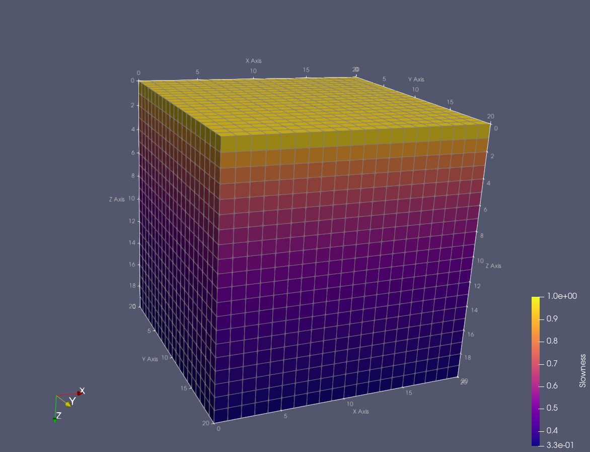
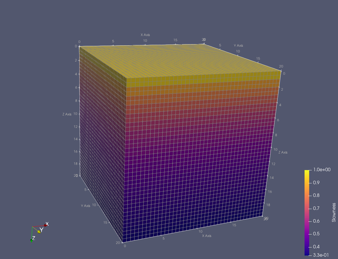
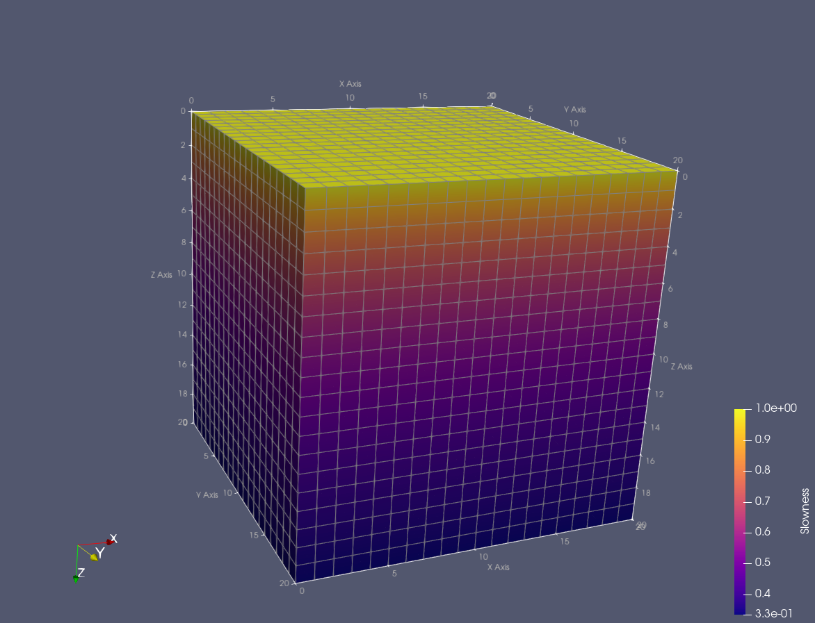
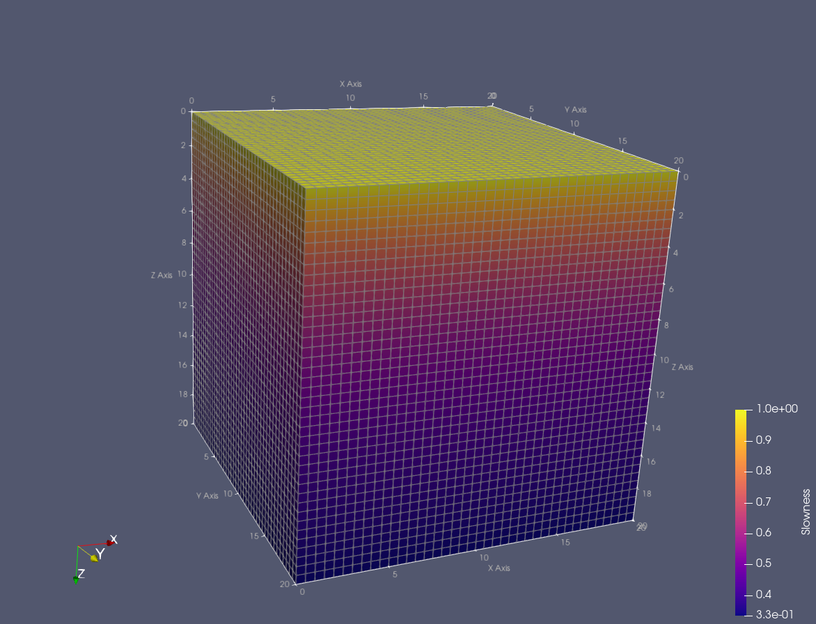
Models
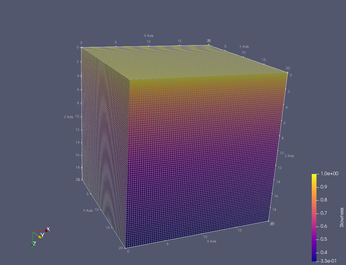
Performance tests were conducted using two different slowness models: a layer-cake model and a vertical gradient model. Analytic solutions exist for both models, which allows accuracy evaluation. Besides, tests were done for three level of discretization: coarse, medium, and fine. The following figures show the models.

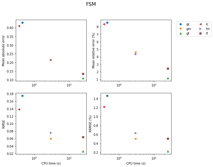
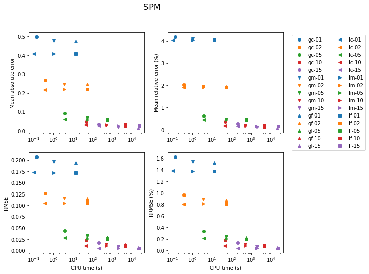
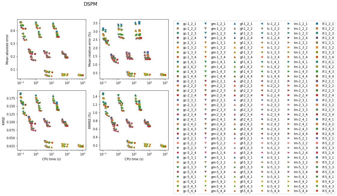
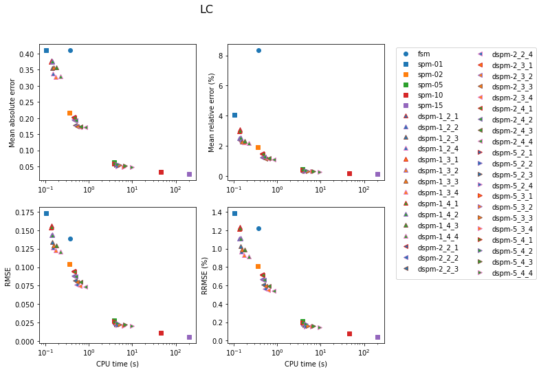
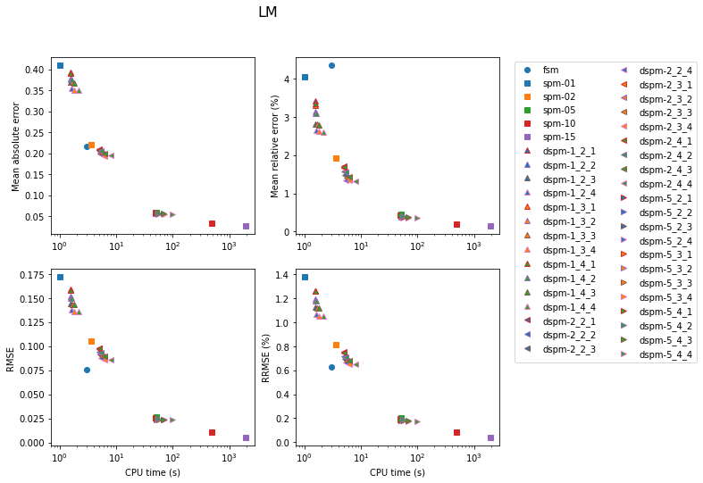
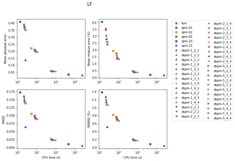
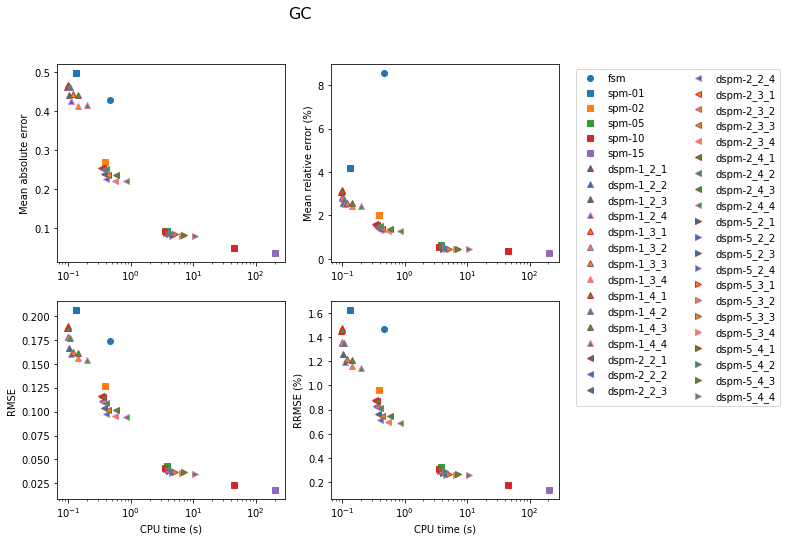
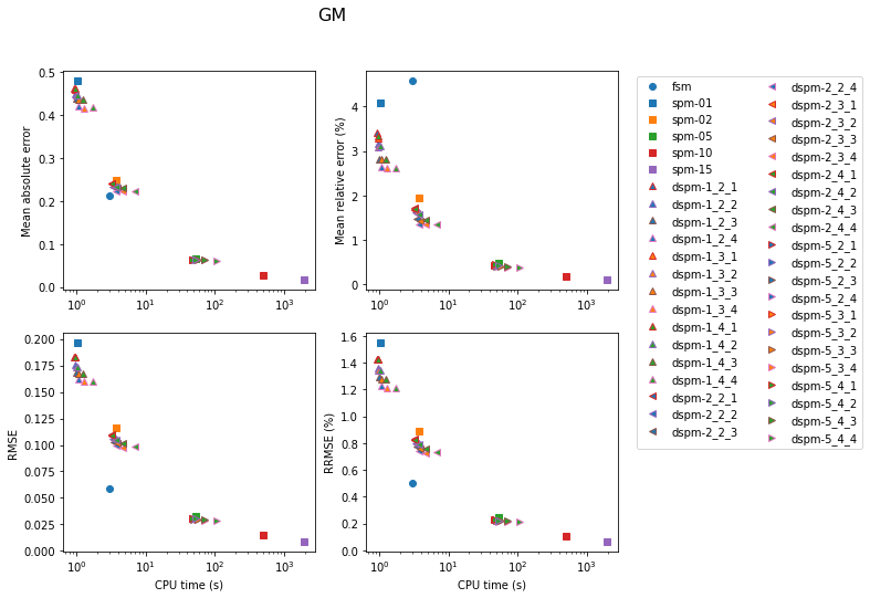
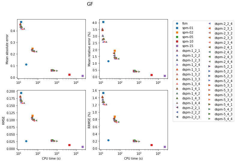
The following figures show the results of the tests. In these figures, models are labelled by two letters: “L” or “G” for layers or gradient, and “C”, “M” or “F” for coarse, medium or fine.
It is important to note that for the layers model, slowness values are assigned to cells, whereas for the gradient model, slowness values are assigned to the nodes of the grid.
Whole-grid accuracy
In this section, the accuracy of the traveltimes computed over the grid nodes (without using the option to update the traveltimes using the raypaths) is evaluated. Error is computed for nodes for which the coordinates are round numbers.
Fast-Sweeping Method
The results are shown first for the FSM. Accuracy is better for the gradient model, except for the coarse models. In the latter case, cells are too large (as thick as the layers) for the solver to yield satisfying accuracy.
Shortest-Path Method
Results for the SPM are shown next. In the legend, the number next to the model label is the number of secondary nodes employed. Increasing this number obviously has an impact on both accuracy and computation time. Using 5 secondary nodes appears to be a good compromise.
Dynamic Shortest-Path Method
Results for the DSPM are shown next, in a rather busy figure. In the legend, the first number next to the model label is the number of secondary nodes, the second number is the number of tertiary nodes, and the last number is the radius of the sphere containing the tertiary nodes around the source.
Results by model
The next set of figures contains the accuracy achieved with the three methods for each model. In all cases, the lowest errors are obtained with the SPM with 15 secondary nodes (at the cost of very high computation time). For the gradient model, the FSM is very competitive for the medium and fine models. Otherwise, the DSPM often appears to offer a good compromise.
2D Rectilinear Grids – OpenCL GPU Speed-up
The OpenCL GPU implementation of the Fast-Sweeping Method (FSM) is available
for 2D rectilinear grids through the classes Grid2Drcfs_OpenCL (cell
slowness) and Grid2Drnfs_OpenCL (node slowness), both exposed via the
Grid2d factory with method='FSM' and fsm_gpu=True. An equivalent
implementation exists for 3D rectilinear grids via the Grid3d factory.
The speed-up over the CPU implementation was measured on homogeneous square
grids of increasing size using single-precision arithmetic (dtype=np.float32).
The source was placed at the grid centre; timing was taken after a warm-up
call that triggers OpenCL kernel compilation. Three repetitions were run at
each size; the minimum is reported.
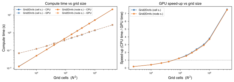
The table below summarises the results:
Grid size N × N |
CPU |
GPU |
Speed-up |
CPU |
GPU |
Speed-up |
|---|---|---|---|---|---|---|
50 × 50 |
0.013 |
0.070 |
0.2× |
0.012 |
0.070 |
0.2× |
100 × 100 |
0.051 |
0.123 |
0.4× |
0.050 |
0.123 |
0.4× |
150 × 150 |
0.114 |
0.180 |
0.6× |
0.113 |
0.180 |
0.6× |
200 × 200 |
0.202 |
0.250 |
0.8× |
0.202 |
0.249 |
0.8× |
300 × 300 |
0.456 |
0.367 |
1.2× |
0.455 |
0.371 |
1.2× |
400 × 400 |
0.813 |
0.505 |
1.6× |
0.811 |
0.526 |
1.5× |
500 × 500 |
1.271 |
0.636 |
2.0× |
1.265 |
0.650 |
1.9× |
600 × 600 |
1.834 |
0.761 |
2.4× |
1.828 |
0.786 |
2.3× |
800 × 800 |
3.270 |
1.083 |
3.0× |
3.254 |
1.114 |
2.9× |
1 000 × 1 000 |
5.137 |
1.354 |
3.8× |
5.105 |
1.381 |
3.7× |
2 000 × 2 000 |
20.643 |
2.736 |
7.5× |
20.629 |
2.759 |
7.5× |
The GPU overhead (kernel launch, host–device transfers) makes the GPU path slower than the CPU for grids smaller than roughly 250 × 250 cells. Beyond that the speed-up grows steadily, reaching 7.5× at 2 000 × 2 000 cells (4 million cells) for both the cell-slowness and node-slowness variants. The two variants exhibit nearly identical timing at every grid size.