Algorithms

ttcrpy contains implementations of three raytracing algorithms.

Shortest-Path

In the shortest path method (SPM), a grid of nodes is used to build a graph by connecting each node to its neighbours. The connections within the graph are assigned a length equal to the traveltime along it. Hence, by virtue of Fermat’s principle which states that a seismic ray follows the minimum traveltime curve, the shortest path between two points within the graph can be seen as an approximation of the raypath.

The SPM algorithm proceeds as follows. After construction of the graph, all nodes are initialized to infinite time except the source nodes which are assigned their “time zero” values. A priority queue is then created and all source nodes are pushed into it. Priority queues are a type of container specifically designed such that its first element is always the one with highest priority, according to some strict weak ordering condition. In our case, the highest priority is attributed to the node having the smallest traveltime value. The traveltime is computed for all nodes connected to the earliest source node, the traveltime value at those nodes is updated with their new value, the parent node is set to the source node, and these nodes then are pushed into the queue. Then, the node with highest priority is popped from the queue, and the traveltime is computed at all nodes connected to it except the node parent. The traveltime and parent values are updated if the traveltime is lower than the one previously assigned, and the nodes not already in the queue are pushed in. This process is repeated until the queue is empty.

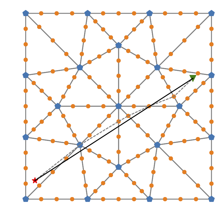
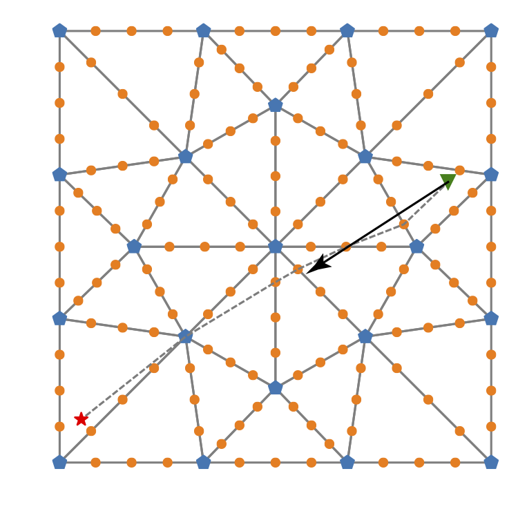
One particular aspect of the ttcrpy implementation is the concept of primary and secondary nodes. Primary nodes are located at the vertexes of the cells, and secondary nodes are surrounding the cells on the edges and faces. In 2D, only secondary edge nodes are introduced. Using secondary nodes allows improving the accuracy and angular coverage of the discrete raypaths. The raypath, however, is an approximation which may deviate from the true raypath, as shown in the figure below which illustrates the case for a homogeneous model.

Dynamic Shortest-Path

Using secondary nodes can be memory and computationally demanding in 3D. With the dynamic variant of the Shortest-Path, the density of secondary nodes is intentionally set to a low value, and tertiary nodes are added to increase the density in the vicinity of the source.

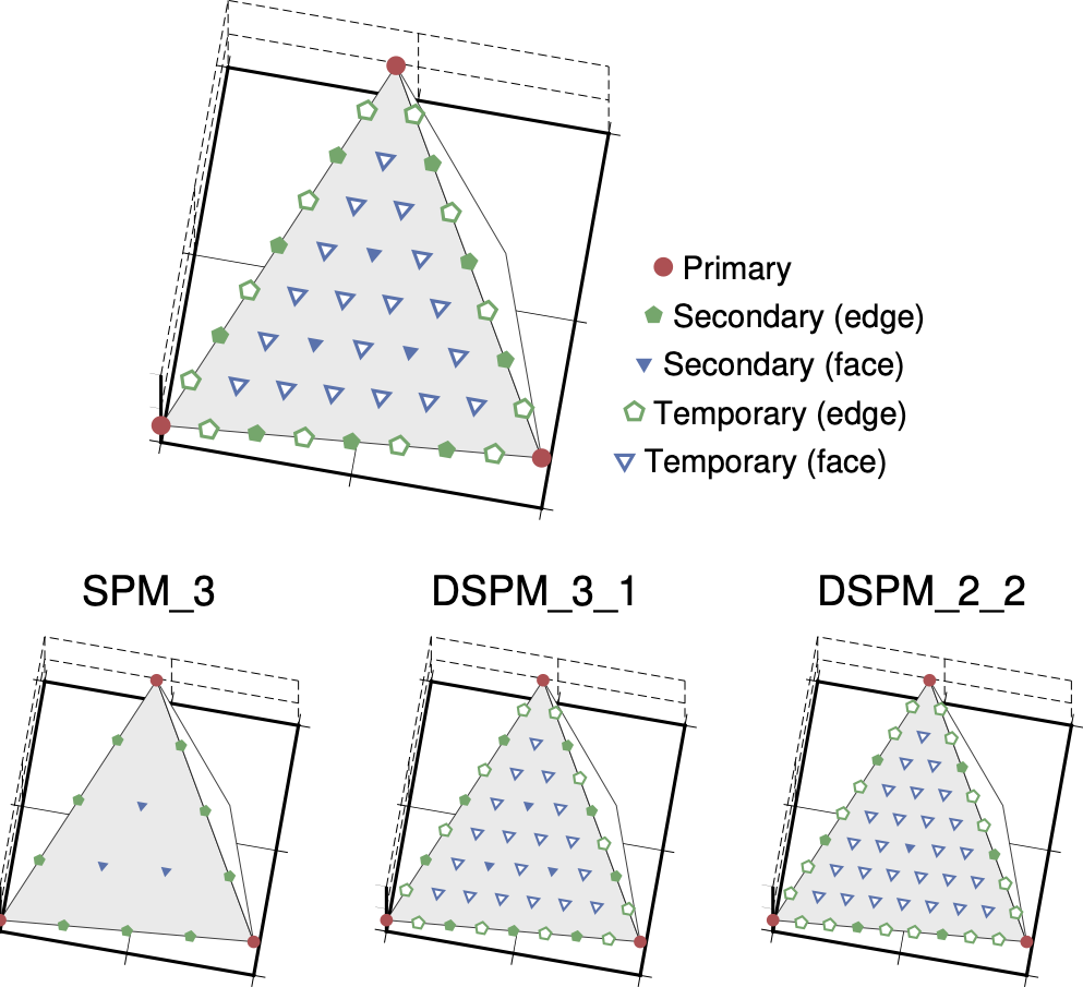
In ttcrpy, tertiary nodes are placed within a sphere centered on the source. Tests have shown that a radius of about three times the mean cell edge length provides a good compromise between accuracy and computation time.

Fast-Sweeping

The Fast-Sweeping Method avoids the requirement to maintain a sorted list of nodes which can be time consuming and resource intensive. The method relies on Gauss-Seidel iterations to propagate the wave front. At each iteration, all the domain nodes are visited and convergence is reached for nodes along characteristic curves parallel to sweeping directions. The causality is ensured by using several Gauss-Seidel iterations with different directions so that all characteristic curves are scanned.

Raypath computation

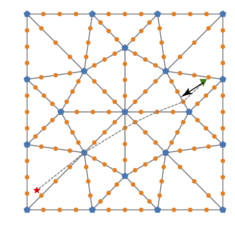
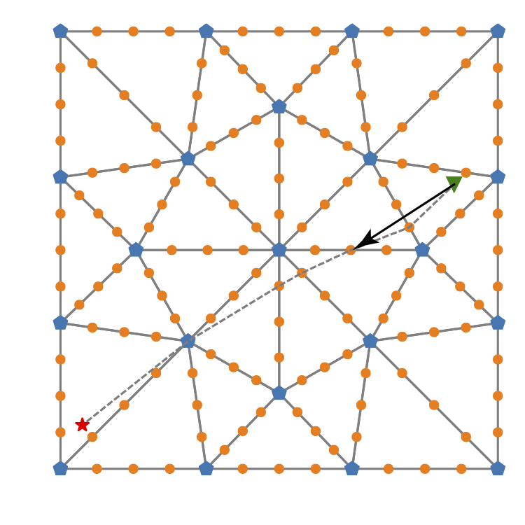
Contrary to the SPM and DSPM, the FSM algorithm does not store raypath segments in memory. When raypaths are needed, they must be computed in a second step. The approach implemented in ttcrpy is to follow the steepest travel time gradient, from the receiver to the source, as illustrated in the figure below.

Computing traveltimes from raypaths

With all three algorithms presented above, traveltimes are computed at all grid nodes. In older version of ttcrpy, we used to interpolate traveltimes at the receivers coordinates and return the interpolated values. We have observed however that results are more accurate if traveltimes are computed in a subsequent step, in which raypaths are computed from the gradient of the traveltimes (as is done with the FSM when raypaths are needed), and traveltimes integrated along the raypaths.

Computing traveltime from raypaths is available as an option for the fast-sweeping and dynamic shortest-path methods. Because the computational cost of the second step is small in comparison to computing traveltime at the grid nodes, the option is activated by default in 3D. We have observed however that for some model with very complex velocity distributions, convergence issues might arise with this option activated, and we suggest to use the SPM method in the latter case. By design, SPM implementations do not include that option, and traveltimes and raypaths are always computed with values at grid nodes.

We have also observed that convergence issues arise when sources or receivers are in the cells at the edges of the modeling domain. For that reason, special care should be put when defining input models and parameters.